MIOpen につながるやさしい入門
A gentle introduction connected to MIOpen
イメージでわかる深層学習
Visual Deep Learning
「AI が画像を認識する」とき、内部では何が起きているのでしょうか。このページでは、ニューラルネット・畳み込み・フィルタ をイメージで説明し、そこから MIOpen が何をしているのか、なぜ solver が複数存在するのかをつなげます。
What actually happens inside AI when it recognises an image? This page explains neural networks, convolution, and filters through images and analogies, then connects them to what MIOpen does and why multiple solvers exist.
まずこれだけ
The essentials
行列変換を何層も重ねた仕組み
Many layers of matrix transforms stacked together
小さい窓で画像をなぞって特徴を探す
Scanning an image with a small window to find features
「どんな特徴を探すか」を決める小さな行列
A small matrix that decides what feature to look for
AMD GPU で畳み込みを担当するライブラリ
The library that handles convolution on AMD GPUs
GPU の能力に合った計算手順を選ぶ仕組み
A mechanism that picks the right computation method for each GPU
ニューラルネットってなに?
What is a neural network?
前のページ(線形代数)で、行列をかける=数字の並びを変換することを説明しました。ニューラルネットワーク(Neural Network / NN)は、この変換を何層も重ねた仕組みです。
The previous page (linear algebra) showed that multiplying by a matrix = transforming a row of numbers. A neural network simply stacks many such transformations in layers.
各層では「変換+非線形な絞り込み」をおこない、それを繰り返すことで、最初はただの数字の集まりだったデータが、最終的に「これは猫」「これは犬」という判断に変わります。
Each layer applies a transform followed by a non-linear squeeze, and repeating this turns a raw collection of numbers into a judgment like "this is a cat" or "this is a dog."
層を重ねるほど「抽象的な特徴」を扱えるようになる
Deeper layers handle increasingly abstract features
漢字を読むとき、最初は「線の組み合わせ」に見えます。次第に「部首」として認識し、最終的に「この字は"山"だ」とわかります。ニューラルネットはこの過程を数値で行います。
When learning to read kanji, you first see "combinations of lines," then recognise radicals, then finally know "this character means mountain." A neural network performs exactly this progression with numbers.
畳み込みってなに?
What is convolution?
全結合のニューラルネットでは、画像の全ピクセルを一度に扱います。しかし画像には「近いピクセルどうしが関係している」という性質があります。端っこ・線・模様は、局所的な範囲に現れるからです。
A fully connected network processes all pixels at once. But images have a key property: nearby pixels relate to each other. Edges, lines, and textures appear in local regions.
そこで「畳み込み」は、小さい窓(フィルタ)を画像の上でずらしながら、その窓の範囲だけを計算するという方法をとります。
Convolution therefore uses a small window (filter) that slides across the image, computing only within that window at each step.
画像の上で小さな虫眼鏡を左から右へ、上から下へとゆっくり動かすことを想像してください。虫眼鏡の中だけを見て「ここに縦線はあるか?」「ここに角はあるか?」と確認していきます。これが畳み込みのイメージです。
Imagine slowly moving a tiny magnifying glass across an image, left to right, top to bottom. At each position you ask only "is there a vertical edge here?" or "is there a corner here?" That is the image of convolution.
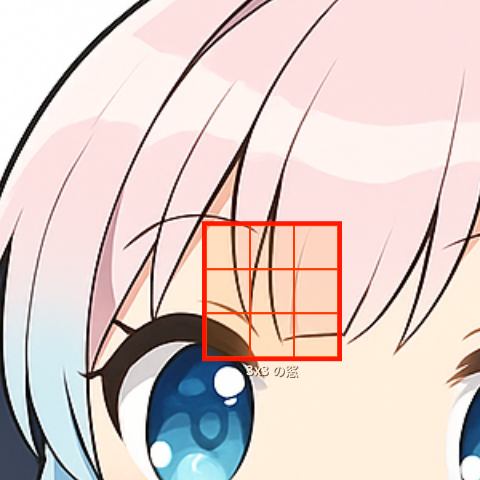
(3×3 の窓で観察中) Original image
(3×3 window scanning)
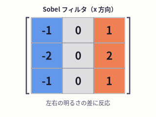
左右の明るさの差を計算 Sobel filter (x-direction)
computes left–right brightness diff
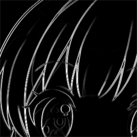
(境界線だけ白く残る) Feature map
(only edges appear white)
左が暗く・右が明るい境界に強く反応 — 数字の符号(−/+)がその仕組みを決めている Responds strongly where left is dark and right is bright — the sign pattern (−/+) encodes this logic
Sobel フィルタ(x 方向)は、左右の明るさの差を計算して、縦方向の境界線を強調します。 The x-direction Sobel filter computes left-right brightness differences and highlights vertical edges.
Sobel フィルタのしくみ — なぜその数字?
How the Sobel filter works — why those numbers?
シーソーのイメージで考えてみましょう。フィルタを窓の上に重ねたとき、左の列はマイナス(暗い側)、右の列はプラス(明るい側) として働きます。真ん中の列は 0 — これは支点にあたる場所で、スコアの計算には参加しません。
Think of it as a seesaw. When the filter is placed on the window, the left column acts as the minus side (dark) and the right column as the plus side (bright). The center column is 0 — it's the pivot, and plays no role in the score.
左と右で明るさが同じなら、マイナスとプラスが打ち消し合って 合計 ≈ 0(境界なし)。左が暗くて右が明るい「段差」があれば、プラス側だけ大きくなって 合計が正の大きな値 になります。
If left and right are equally bright, the minus and plus cancel out → total ≈ 0 (no edge). If left is dark and right is bright — a real step — only the plus side is large → large positive total.
具体的な数字で確かめてみましょう。窓の左側が暗い(輝度 10)、右側が明るい(輝度 200)場合:
Let's verify with real numbers. Suppose the left side of the window is dark (brightness 10) and the right side is bright (brightness 200):
⚠️ ここでの「×」は、前のページで見た行列の掛け算(ヨコ×タテ)とは別の計算です。
3×3 の画像とフィルタをぴったり重ねて、同じ場所どうしを掛け算し、最後に全部足します。
⚠️ The "×" here is not regular matrix multiplication (row × column).
Instead, the 3×3 image patch and filter are laid on top of each other; matching positions are multiplied, then all nine products are summed.
| 10 | 10 | 200 |
| 10 | 10 | 200 |
| 10 | 10 | 200 |
どうし
positions
| −1 | 0 | +1 |
| −2 | 0 | +2 |
| −1 | 0 | +1 |
この「760」という大きな正の値が、特徴マップの明るい白い点として記録されます。
This large positive value (760) is what gets recorded as a bright white dot in the feature map.
合計値の符号(プラス・マイナス・ゼロ)が意味すること:
What the sign of the total means:
- 正(+) Positive (+) 左が暗く、右が明るい。左→右へ明るくなる境界。 Left is dark, right is bright. Brightness rises left-to-right.
- 負(−) Negative (−) 左が明るく、右が暗い。右→左へ明るくなる境界。 Left is bright, right is dark. Brightness rises right-to-left.
- ゼロ付近 Near zero 左右の明るさがほぼ同じ。境界線なし。 Left and right brightness are nearly equal. No edge.
フィルタってなに?
What is a filter?
フィルタ(カーネルとも呼ぶ)は、「どんな特徴を探すか」を決める小さな行列です。
A filter (also called a kernel) is a small matrix that decides what feature to look for.
手で設計することもできますが、深層学習では フィルタの中身(重み)を訓練によって自動で決めるのが特徴です。モデルが「猫を見分けるのに役立つ特徴」を自分で学んでいきます。(訓練の流れは 学習の流れ ページで解説しています。)
Filters can be designed by hand, but the key feature of deep learning is that filter weights are determined automatically through training. The model learns by itself which features help distinguish a cat. (See Visual Guide to the Training Flow for how training works.)
畳み込み層には複数のフィルタがあり、それぞれが異なる特徴を探します。最初の層では「端っこ・線」、深い層では「目・耳」のような複雑な部品を探すようになります。
A convolutional layer has many filters, each looking for a different feature. Early layers find "edges and lines"; deeper layers find complex parts like "eyes and ears."
畳み込みを重ねるほど抽象度の高い特徴を扱える(CNN = 畳み込みニューラルネット)
Stacking convolutions handles increasingly abstract features (CNN = Convolutional Neural Network)
畳み込みの先へ — Attention と LLM
Beyond convolution — Attention and LLMs
畳み込みは「近くの情報を見る」のが得意ですが、文章では遠くの単語どうしの関係もとても重要です。たとえば「太郎はケーキを食べた。そのあと彼は寝た」の「彼」が誰を指すかは、前の文まで遡らないとわかりません。
Convolution excels at nearby patterns, but language requires relationships between distant words too. For example, knowing who "he" refers to in "Taro ate the cake. Then he slept" requires reaching back to an earlier sentence.
そのため、現在の大規模言語モデル(LLM)では、畳み込みよりも Attention(注意機構) が中心的な仕組みになっています。Attention は文中の全単語を同時に参照し、関係が深い単語ほど強く注目する仕組みです。GPT・BERT・LLaMA など現代の LLM はほぼすべて、Attention を積み重ねた Transformer アーキテクチャを使っています。
That's why today's large language models (LLMs) rely on Attention rather than convolution. Attention looks at all words in a sentence simultaneously, weighting the most relevant ones more strongly. GPT, BERT, LLaMA and virtually all modern LLMs use the Transformer architecture, which stacks Attention layers.
Attention の詳しい説明は別ページで
Attention explained in depth — on a separate page
Query / Key / Value の役割、softmax の意味、Transformer のしくみ、MIOpen との接続は、専用の入門ページ「イメージでわかる Attention」で段階的に説明しています。
The roles of Query / Key / Value, what softmax does, how Transformer works, and the connection to MIOpen are all explained step-by-step in the dedicated intro page "Visual Attention for Beginners."
イメージでわかる Attention を読む → Read: Visual Attention for Beginners →MIOpen ってなに?
What is MIOpen?
MIOpen は、AMD GPU で畳み込み・行列演算・プーリングなど DNN の基本計算を高速に実行するためのライブラリです。
MIOpen is AMD's library for running DNN building blocks — convolution, matrix operations, pooling, etc. — at full GPU speed.
PyTorch などの AI フレームワークから「畳み込みを実行してください」と呼ばれると、MIOpen がその GPU に合った最適な計算手順(solver)を選んで実行します。
When an AI framework like PyTorch says "run a convolution," MIOpen selects the optimal computation method (solver) for the specific GPU and executes it.
MIOpen は「要求を受けて → solver を選んで → GPU で実行する」仲介役
MIOpen is the intermediary that "receives requests → selects a solver → executes on GPU"
なぜ solver がたくさんあるの?
Why are there so many solvers?
同じ「畳み込み」でも、GPU の世代・命令セット・入力の形・データ型によって、最も速い計算手順が変わります。MIOpen はそれぞれに対応した solver を登録しており、実行前に「この GPU でこの入力に使えるか?」(IsApplicable())を確認して最適なものを選びます。
Even for the same "convolution," the fastest computation method varies depending on the GPU generation, instruction set, input shape, and data type. MIOpen registers a solver for each case and checks "can this solver run on this GPU with this input?" (IsApplicable()) before selecting the best one.
「東京から大阪に行く」方法は、新幹線・飛行機・在来線・バスなど複数あります。最も速い手段は、時間帯・予算・出発地によって変わります。solver はその「移動手段のリスト」です。使える手段があれば使い、なければ次の手段を試します。
There are many ways to get from Tokyo to Osaka — shinkansen, plane, local train, bus. The fastest option depends on timing, budget, and starting point. Solvers are that list of travel options: use the best available one and fall back to the next if the first is unavailable.
| Solver | 得意なこと | gfx900 | gfx908+ | Solver | Strength | gfx900 | gfx908+ |
|---|---|---|---|---|---|---|---|
| MLIR iGEMM | MLIR コンパイラ経由の高速 GEMM | ✗ 除外 | ✓ | Fast GEMM via MLIR compiler | ✗ excluded | ✓ | |
| XDLops / CK | 行列演算専用命令(xdlops)を使う | ✗ 命令なし | ✓ | Uses dedicated xdlops matrix instructions | ✗ no xdlops | ✓ | |
| Winograd | 小カーネル畳み込みの演算量削減 | ✓ 動作 | ✓ | Reduces operations for small-kernel convolutions | ✓ works | ✓ | |
| ASM v4r1 | 手書きアセンブリで最適化した経路 | ✓ 動作 | ✓ | Hand-written assembly optimised path | ✓ works | ✓ | |
| Naive / Reference | どの GPU でも必ず動く汎用経路 | ✓ 常に利用可 | ✓ | Generic path guaranteed to work on any GPU | ✓ always | ✓ |
gfx900 で何が使えて、何がつらいの?
What works on gfx900 and what is hard?
gfx900(Vega 世代)は 2017 年の GPU です。最近の GPU にある「行列計算のための専用の近道」の一部を持っていません。名前で言うと xdlops や dot4 です。
gfx900 (Vega generation) is a 2017 GPU. It has neither xdlops (dedicated matrix instructions) nor dot4 (INT8 multiply-accumulate).
そのため、MLIR iGEMM と XDLops 系の solver は使えません。しかし Winograd / ASM v4r1 は今も動作し、MIOpen の Naive solver は常に利用できます。また、Perf DB(性能チューニング済みパラメータ集)に gfx900 向けの 169,182 行のエントリが ROCm 7.2 に収録されており、これが動作を支えています。
As a result, MLIR iGEMM and XDLops solvers are unavailable. But Winograd and ASM v4r1 still work, and the Naive solver is always available. The Perf DB (pre-tuned parameter database) also ships 169,182 gfx900 entries in ROCm 7.2, which underpins continued operation.
速い道は使えないが、使える solver が残っているため計算は成立する
Fast paths are blocked, but remaining solvers keep computation viable
- MIOpen MLIR iGEMM は commit
2407d2f(2021-12-22)で gfx900 を明示除外 - Winograd・ASM v4r1 は
IsApplicable()を通過し、現在も動作する - INT8 は dot4 命令がないため Naive solver のみ(実機逆アセンブルで確認)
- gfx900 向け Perf DB エントリ 169,182 行が ROCm 7.2 に同梱
- MIOpen MLIR iGEMM explicitly excluded gfx900 in commit
2407d2f(2021-12-22) - Winograd and ASM v4r1 pass
IsApplicable()and remain functional - INT8 uses Naive solver only due to absent dot4 instructions (confirmed by disassembly)
- 169,182 gfx900 Perf DB entries ship with ROCm 7.2
まとめ
Summary
- ニューラルネットは行列変換の積み重ね。畳み込みはその中で「局所特徴を探す」専門の層
- フィルタが「何の特徴を探すか」を決め、訓練で自動的に最適化される
- MIOpen は AMD GPU で畳み込みを担当するライブラリ。GPU に合った solver を選んで実行する
- gfx900 は速い solver が使えないが、Winograd / ASM v4r1 / Naive で動作が継続している
- A neural network stacks matrix transforms; convolution is the specialised layer that searches for local features
- Filters decide what feature to look for and are optimised automatically during training
- MIOpen is the AMD GPU convolution library; it selects a GPU-appropriate solver and runs it
- gfx900 cannot use the fast solvers, but Winograd, ASM v4r1, and Naive keep it working